使用Neura动力系统建模l ODE

Open Live Script

This example shows how to train a neural network with neural ordinary differential equations (ODEs) to learn the dynamics of a physical system.

Neural ODEs [1] are deep learning operations defined by the solution of an ODE. More specifically, neural ODE is an operation that can be used in any architecture and, given an input, defines its output as the numerical solution of the ODE

$y^{'} = f (t, y, θ)$

for the time horizon $(t_{0}, t_{1})$ and the initial condition $y (t_{0}) = y_{0}$ . The right-hand side $f (t, y, θ)$ of the ODE depends on a set of trainable parameters $θ$ , which the model learns during the training process. In this example, $f (t, y, θ)$ is modeled with a model function containing fully connected operations and nonlinear activations. The initial condition $y_{0}$ is either the input of the entire architecture, as in the case of this example, or is the output of a previous operation.

This example shows how to train a neural network with neural ODEs to learn the dynamics $x$ of a given physical system, described by the following ODE:

$x^{'} = A x$ ,

where $A$ is a 2-by-2 matrix.

The neural network of this example takes as input an initial condition and computes the ODE solution through the learned neural ODE model.

The neural ODE operation, given an initial condition, outputs the solution of an ODE model. In this example, specify a block with a fully connected layer, a tanh layer, and another fully connected layer as the ODE model.

In this example, the ODE that defines the model is solved numerically with the explicit Runge-Kutta (4,5) pair of Dormand and Prince [2]. The backward pass uses automatic differentiation to learn the trainable parameters $θ$ by backpropagating through each operation of the ODE solver.

The learned function $f (t, y, θ)$ is used as the right-hand side for computing the solution of the same model for additional initial conditions.

Synthesize Data of Target Dynamics

Define the target dynamics as a linear ODE model $x^{'} = A x$ , withx0as its initial condition, and compute its numerical solutionxTrainwithode45in the time interval[0 15]. To compute an accurate ground truth data, set the relative tolerance of theode45numerical solver to $10^{- 7}$ . Later, you use the value ofxTrainas ground truth data for learning an approximated dynamics with a neural ODE model.

x0 = [2; 0]; A = [-0.1 -1; 1 -0.1]; trueModel = @(t,y) A*y; numTimeSteps = 2000; T = 15; odeOptions = odeset(RelTol=1.e-7); t = linspace(0, T, numTimeSteps); [~, xTrain] = ode45(trueModel, t, x0, odeOptions); xTrain = xTrain';

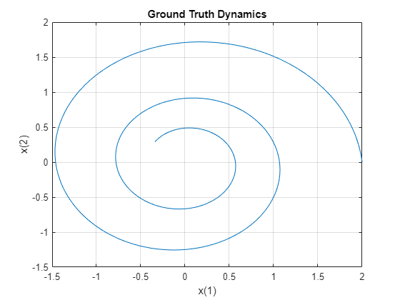
Visualize the training data in a plot.

figure plot(xTrain(1,:),xTrain(2,:)) title("Ground Truth Dynamics") xlabel("x(1)") ylabel("x(2)") gridon

Define and Initialize Model Parameters

The model function consists of a single call todlode45to solve the ODE defined by the approximated dynamics $f (t, y, θ)$ for 40 time steps.

neuralOdeTimesteps = 40; dt = t(2); timesteps = (0:neuralOdeTimesteps)*dt;

Define the learnable parameters to use in the call todlode45and collect them in the variableneuralOdeParameters. The functioninitializeGlorottakes as input the size of the learnable parametersszand the number of outputs and number of inputs of the fully connected operations, and returns adlarrayobject with underlying typesinglewith values set using Glorot initialization. The functioninitializeZerostakes as input the size of the learnable parameters, and returns the parameters as adlarrayobject with underlying typesingle. The initialization example functions are attached to this example as supporting files. To access these functions, open this example as a live script. For more information about initializing learnable parameters for model functions, seeInitialize Learnable Parameters for Model Function.

Initialize the parameters structure.

neuralOdeParameters = struct;

Initialize the parameters for the fully connected operations in the ODE model. The first fully connected operation takes as input a vector of sizestateSizeand increases its length tohiddenSize. Conversely, the second fully connected operation takes as input a vector of lengthhiddenSizeand decreases its length tostateSize.

stateSize = size(xTrain,1); hiddenSize = 20; neuralOdeParameters.fc1 = struct; sz = [hiddenSize stateSize]; neuralOdeParameters.fc1.Weights = initializeGlorot(sz, hiddenSize, stateSize); neuralOdeParameters.fc1.Bias = initializeZeros([hiddenSize 1]); neuralOdeParameters.fc2 = struct; sz = [stateSize hiddenSize]; neuralOdeParameters.fc2.Weights = initializeGlorot(sz, stateSize, hiddenSize); neuralOdeParameters.fc2.Bias = initializeZeros([stateSize 1]);

Display the learnable parameters of the model.

neuralOdeParameters.fc1

ans =struct with fields:Weights: [20×2 dlarray] Bias: [20×1 dlarray]

neuralOdeParameters.fc2

ans =struct with fields:Weights: [2×20 dlarray] Bias: [2×1 dlarray]

Define Neural ODE Model

Create the functionodeModel, listed in theODE Modelsection of the example, which takes as input the time input (unused), the corresponding solution, and the ODE function parameters. The function applies a fully connected operation, a tanh operation, and another fully connected operation to the input data using the weights and biases given by the parameters.

Define Model Function

Create the functionmodel, listed in theModel Functionsection of the example, which computes the outputs of the deep learning model. The functionmodeltakes as input the model parameters and the input data. The function outputs the solution of the neural ODE.

Define Model Loss Function

Create the functionmodelLoss, listed in theModel Loss Functionsection of the example, which takes as input the model parameters, a mini-batch of input data with corresponding targets, and returns the loss and the gradients of the loss with respect to the learnable parameters.

Specify Training Options

指定的选项为亚当的优化。

gradDecay = 0.9; sqGradDecay = 0.999; learnRate = 0.002;

Train for 1200 iterations with a mini-batch-size of 200.

numIter = 1200; miniBatchSize = 200;

Every 50 iterations, solve the learned dynamics and display them against the ground truth in a phase diagram to show the training path.

plotFrequency = 50;

Train Model Using Custom Training Loop

Initialize the training progress plot.

f = figure; f.Position(3) = 2*f.Position(3); subplot(1,2,1) C = colororder; lineLossTrain = animatedline(Color=C(2,:)); ylim([0 inf]) xlabel("Iteration") ylabel("Loss") gridon

Initialize theaverageGradandaverageSqGradparameters for the Adam solver.

averageGrad = []; averageSqGrad = [];

Train the network using a custom training loop.

For each iteration:

Construct a mini-batch of data from the synthesized data with thecreateMiniBatchfunction, listed in theCreate Mini-Batches Functionsection of the example.
Evaluate the model loss and gradients and loss using thedlfevalfunction and themodelLossfunction, listed in theModel Loss Functionsection of the example.
Update the model parameters using theadamupdatefunction.
Update the training progress plot.

numTrainingTimesteps = numTimeSteps; trainingTimesteps = 1:numTrainingTimesteps; plottingTimesteps = 2:numTimeSteps; start = tic;foriter = 1:numIter% Create batch[X, targets] = createMiniBatch(numTrainingTimesteps, neuralOdeTimesteps, miniBatchSize, xTrain);% Evaluate network and compute loss and gradients[loss,gradients] = dlfeval(@modelLoss,timesteps,X,neuralOdeParameters,targets);% Update network[neuralOdeParameters,averageGrad,averageSqGrad] = adamupdate(neuralOdeParameters,gradients,averageGrad,averageSqGrad,iter,...learnRate,gradDecay,sqGradDecay);% Plot losssubplot(1,2,1) currentLoss = double(loss); addpoints(lineLossTrain,iter,currentLoss); D = duration(0,0,toc(start),Format="hh:mm:ss"); title("Elapsed: "+ string(D)) drawnow% Plot predicted vs. real dynamicsifmod(iter,plotFrequency) == 0 || iter == 1 subplot(1,2,2)% Use ode45 to compute the solutiony = dlode45(@odeModel,t,dlarray(x0),neuralOdeParameters,DataFormat="CB"); plot(xTrain(1,plottingTimesteps),xTrain(2,plottingTimesteps),"r--") holdonplot(y(1,:),y(2,:),"b-") holdoffxlabel("x(1)") ylabel("x(2)") title("Predicted vs. Real Dynamics") legend("Training Ground Truth","Predicted") drawnowendend

Evaluate Model

Use the model to compute approximated solutions with different initial conditions.

Define four new initial conditions different from the one used for training the model.

tPred = t; x0Pred1 = sqrt([2;2]); x0Pred2 = [-1;-1.5]; x0Pred3 = [0;2]; x0Pred4 = [-2;0];

Numerically solve the ODE true dynamics withode45for the four new initial conditions.

[~, xTrue1] = ode45(trueModel, tPred, x0Pred1, odeOptions); [~, xTrue2] = ode45(trueModel, tPred, x0Pred2, odeOptions); [~, xTrue3] = ode45(trueModel, tPred, x0Pred3, odeOptions); [~, xTrue4] = ode45(trueModel, tPred, x0Pred4, odeOptions);

Numerically solve the ODE with the learned neural ODE dynamics.

xPred1 = dlode45(@odeModel,tPred,dlarray(x0Pred1),neuralOdeParameters,DataFormat="CB"); xPred2 = dlode45(@odeModel,tPred,dlarray(x0Pred2),neuralOdeParameters,DataFormat="CB"); xPred3 = dlode45(@odeModel,tPred,dlarray(x0Pred3),neuralOdeParameters,DataFormat="CB"); xPred4 = dlode45(@odeModel,tPred,dlarray(x0Pred4),neuralOdeParameters,DataFormat="CB");

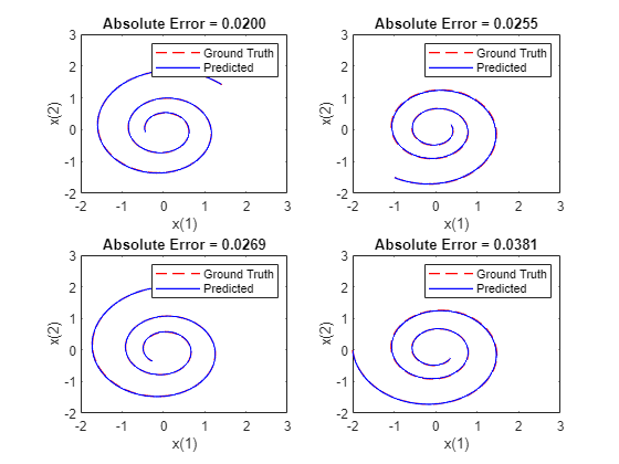
Visualize Predictions

Visualize the predicted solutions for different initial conditions against the ground truth solutions with the functionplotTrueAndPredictedSolutions, listed in thePlot True and Predicted Solutions Functionsection of the example.

figure subplot(2,2,1) plotTrueAndPredictedSolutions(xTrue1, xPred1); subplot(2,2,2) plotTrueAndPredictedSolutions(xTrue2, xPred2); subplot(2,2,3) plotTrueAndPredictedSolutions(xTrue3, xPred3); subplot(2,2,4) plotTrueAndPredictedSolutions(xTrue4, xPred4);

Helper Functions

Model Function

Themodelfunction, which defines the neural network used to make predictions, is composed of a single neural ODE call. For each observation, this function takes a vector of lengthstateSize, which is used as initial condition for solving numerically the ODE with the functionodeModel代表可学的right-hand side $f (t, y, θ)$ of the ODE to be solved, as right hand side and a vector of time pointstspandefining the time at which the numerical solution is output. The function uses the vectortspan为每个observation, regardless of the initial condition, since the learned system is autonomous. That is, theodeModelfunction does not explicitly depend on time.

functionX = model(tspan,X0,neuralOdeParameters) X = dlode45(@odeModel,tspan,X0,neuralOdeParameters,DataFormat="CB");end

ODE Model

TheodeModelfunction is the learnable right-hand side used in the call todlode45. It takes as input a vector of sizestateSize, enlarges it so that it has lengthhiddenSize, and applies a nonlinearity functiontanh. Then the function compresses the vector again to have lengthstateSize.

functiony = odeModel(~,y,theta) y = tanh(theta.fc1.Weights*y + theta.fc1.Bias); y = theta.fc2.Weights*y + theta.fc2.Bias;end

Model Loss Function

This function takes as inputs a vectortspan, a set of initial conditionsX0, the learnable parametersneuralOdeParameters, and target sequencestargets. It computes the predictions with themodelfunction, and compares them with the given targets sequences. Finally, it computes the loss and the gradient of the loss with respect to the learnable parameters of the neural ODE.

function[loss,gradients] = modelLoss(tspan,X0,neuralOdeParameters,targets)% Compute predictions.X = model(tspan,X0,neuralOdeParameters);% Compute L1 loss.loss = l1loss(X,targets,NormalizationFactor="all-elements",DataFormat="CBT");% Compute gradients.gradients = dlgradient(loss,neuralOdeParameters);end

Create Mini-Batches Function

ThecreateMiniBatchfunction creates a batch of observations of the target dynamics. It takes as input the total number of time steps of the ground truth datanumTimesteps, the number of consecutive time steps to be returned for each observationnumTimesPerObs, the number of observationsminiBatchSize, and the ground truth dataX.

function[x0, targets] = createMiniBatch(numTimesteps,numTimesPerObs,miniBatchSize,X)% Create batches of trajectories.s = randperm(numTimesteps - numTimesPerObs, miniBatchSize); x0 = dlarray(X(:, s)); targets = zeros([size(X,1) miniBatchSize numTimesPerObs]);fori = 1:miniBatchSize targets(:, i, 1:numTimesPerObs) = X(:, s(i) + 1:(s(i) + numTimesPerObs));endend

Plot True and Predicted Solutions Function

TheplotTrueAndPredictedSolutionsfunction takes as input the true solutionxTrue, the approximated solutionxPredcomputed with the learned neural ODE model, and the corresponding initial conditionx0Str. It computes the error between the true and predicted solutions and plots it in a phase diagram.

functionplotTrueAndPredictedSolutions(xTrue,xPred) xPred = squeeze(xPred)'; err = mean(abs(xTrue(2:end,:) - xPred),"all"); plot(xTrue(:,1),xTrue(:,2),"r--",xPred(:,1),xPred(:,2),"b-",LineWidth=1) title("Absolute Error = "+ num2str(err,"%.4f")包含("x(1)") ylabel("x(2)") xlim([-2 3]) ylim([-2 3]) legend("Ground Truth","Predicted")end

[1] Chen, Ricky T. Q., Yulia Rubanova, Jesse Bettencourt, and David Duvenaud. “Neural Ordinary Differential Equations.” Preprint, submitted December 13, 2019. https://arxiv.org/abs/1806.07366.

[2] Shampine,和马克·w·劳伦斯•F。摘要。”The MATLAB ODE Suite.” SIAM Journal on Scientific Computing 18, no. 1 (January 1997): 1–22. https://doi.org/10.1137/S1064827594276424.